Orthomode Transducers: Part 6 – Testing Back-to-Back OMTs

David W. Porterfield, PhD
Founder, Micro Harmonics

This is the sixth blog in a series on orthomode transducers. So far, we have introduced orthomode transducers (OMTs) and their applications [1], explored several common OMT architectures [2], outlined the key performance parameters used to evaluate them [3], explained how to obtain useful RF test data using a simple short circuit termination [4], and covered RF testing methods using a matched load on the common mode port [5].

In this blog we will describe RF testing methods using a pair of OMTs attached at the common mode port. This back-to-back configuration can yield comprehensive data on the OMT characteristics.

OMT Description

OMTs have three waveguide ports. Two of the ports support a single TE10 propagating mode in a rectangular waveguide. The third port, the common mode port, supports two orthogonal propagating modes. The common mode waveguide can have a square cross-section supporting orthogonal TE10 and TE01 modes or a circular cross-section supporting a pair of degenerate orthogonal TE11 modes.

Figure 1 shows a simplified sketch of an OMT. Port 1 on the axial waveguide and port 2 on the lateral waveguide each support a single TE10 mode. The common mode waveguide supports two polarizations designated as vertical (V) and horizontal (H). The two modes can be treated as two distinct ports, port 3 (V) and port 4 (H). The vertical (V) and horizontal (H) designations simply help us keep track of the associated polarizations. An ideal OMT couples 100% of the vertically polarized signal between ports 1 (V) and port 3 (V) and 100% of the horizontally polarized signal between ports 2 (H) and port 4 (H).

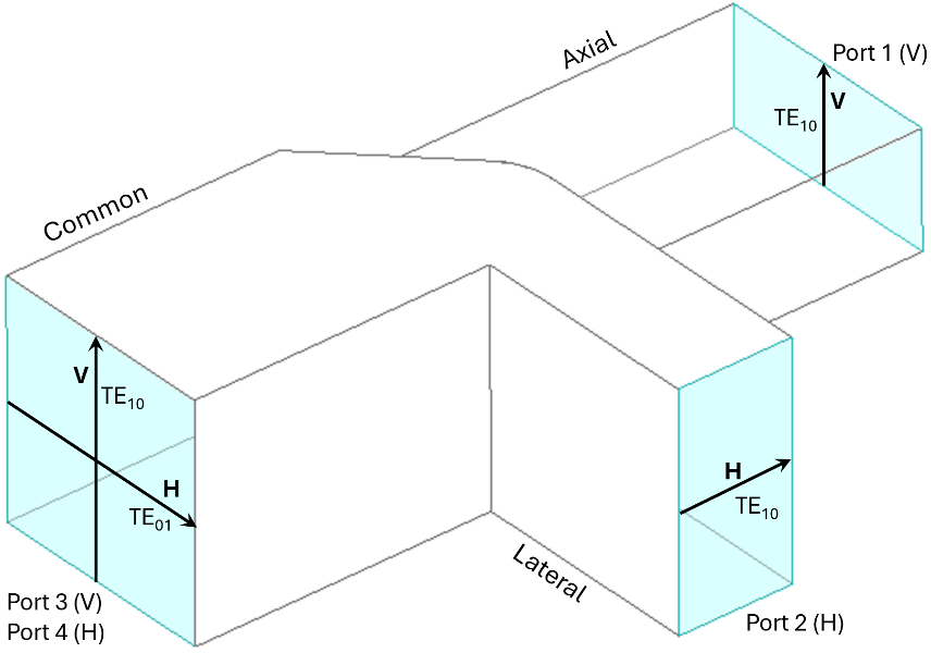
Figure 1 – Simplified asymmetric T-Junction OMT with polarization and port designations.

Difficulties of Characterizing OMTs

RF testing of OMTs is complicated by the presence of the common mode port, which supports two orthogonal modes. Vector network analyzers have single-mode test ports. The question is how to handle the common mode port in testing.

Testing Back-to-Back OMTs

The short circuit test described in a previous blog [4] provides useful data for insertion loss and qualitative data for isolation and cross-polarization coupling. The matched load testing described in the previous blog [5] provides accurate data for port reflections and isolation but requires a dual-polarized square waveguide matched load, which is not readily available on the commercial market.

Testing becomes easier and more robust if two or more OMTs are available. The OMTs can be tested in pairs by attaching them to the common mode ports as shown in Figure 2. The two connected OMTs form a four-port device where each port is a rectangular waveguide supporting a single TE10 mode. A common testing procedure would involve terminating two of the ports with matched loads and attaching a vector network analyzer to the remaining two ports via waveguide frequency extenders.

Port reflections S11 and S22 can be measured with a high degree of accuracy by attaching the network analyzer to ports 1 and 2 and terminating ports 3 and 4 with matched loads. In this case, the second OMT (B) functions as a dual-polarized matched load on the common port of the first OMT (A). Similarly, S33 and S44 can be measured by terminating ports 1 and 2. The isolation is given by S12, S21, S34, and S43.

Figure 2 – Two OMTs connected to create a device with four single-mode ports.

Insertion loss S31 and S13 can be measured by attaching the network analyzer to ports 1 and 3 and terminating ports 2 and 4. The measured insertion loss is for the vertical polarization of both OMTs A & B in series and is approximately double the value of the insertion loss of the vertical polarization of a single OMT. Similarly, insertion loss S42 and S24 can be measured by attaching the network analyzer to ports 2 and 4 and terminating ports 1 and 3.

Cross polarization coupling S41 and S14 can be measured by attaching the network analyzer to ports 1 and 4 and terminating ports 2 and 3. There are two paths that a vertically polarized signal incident on port 1 can travel to reach port 4. In the first path, the vertically polarized signal at port 1 is cross-polarization coupled in OMT (A) to the horizontal polarization at the junction between the two OMTs. The horizontally polarized signal then propagates to port 4 incurring a single insertion loss in the horizontal polarization.

In the second path, the vertically polarized signal incident on port 1 couples to the vertical polarization at the junction between the two OMTs, incurring a single vertical insertion loss in OMT (A). The signal is then cross-polarization coupled to port 4 in OMT (B). The S41 measurement is dominated by low cross polarization coupling. The insertion loss can either be ignored or calculated out. A similar argument is made for S14. The remaining cross polarization coupling parameters, S23 and S32, can be measured by attaching the network analyzer to ports 2 and 3 and attaching the terminations to ports 1 and 4.

The connected OMTs will not have the same exact characteristics, so the characteristics of one OMT impacts the measurement of the other. However, network theory shows that if a third OMT is used and a series of tests is performed where the three OMTs are tested and interchanged in every possible configuration, the individual OMT characteristics can be extracted from the data with a high degree of accuracy. A full explanation is beyond the scope of this blog. For a more in depth look at methods for accurately characterizing OMTs, refer to the paper by Alessandro Navarrini and Renzo Nesti [6].

Summary of Back-to-Back OMT Testing

OMTs serve an important function in separating and combining orthogonal polarizations. But OMTs have practical limitations. It is important to understand the desirable characteristics of OMTs including low insertion loss, high isolation, low cross polarization coupling, and low port reflection. It is also important to understand the difficulties in accurately measuring and characterizing OMT performance. The difficulties arise because the OMT common port supports two propagating modes and cannot be connected to a vector network analyzer.

Several RF testing methods were described that vary primarily in how the common mode port is terminated. The various terminations include a short circuit [4], a dual-mode matched load [5], a single mode matched load via a linear taper [5], and back-to-back testing of pairs of OMTs connected at the common port. Each method has strengths and weaknesses in terms of simplicity and accuracy.

At Micro Harmonics, we apply this same attention to RF performance and precision engineering across a wide range of high-frequency solutions, including circulators, isolators, attenuators, and advanced cryogenic millimeter wave components. Our experience designing and testing microwave and millimeter-wave technologies helps support demanding applications where accuracy, stability, and low-loss performance are essential.

References

[1] D. Porterfield, “Orthomode Transducers: Part 1 – Introduction and Applications,” A brief description of orthomode transducers (OMTs) and common applications. https://microharmonics.com/blog/, January 31, 2025.

[2] D. Porterfield, “Orthomode Transducers: Part 2 – Architectures,” A brief description of some of the most common mm-wave OMT architectures. https://microharmonics.com/blog/, May 21, 2025

[3] D. Porterfield, “Orthomode Transducers: Part 3 – Characterization,” A description of important OMT parameters including insertion loss, port reflections, cross-polarization coupling, and isolation. https://microharmonics.com/blog/, 2026

[4] D. Porterfield, “Orthomode Transducers: Part 4 – RF Testing with a Short Circuit Termination,” How to measure insertion loss and qualitatively characterize isolation and cross-polarization coupling using a short circuit termination on the common mode port. https://microharmonics.com/blog/, 2026

[5] D. Porterfield, “Orthomode Transducers: Part 5 – RF Testing with a Matched Load,” How to measure isolation and port reflections using a matched load. https://microharmonics.com/blog/, 2026

[6] Alessandro Navarrini and Renzo Nesti, “Characterization Techniques of Millimeter-Wave Orthomode Transducers (OMTs),” Electronics 2021, Vol 10, Issue 15, 1844, https://doi.org/10.3390/electronics10151844. https://microharmonics.com/blog/, May 21, 2025