
Orthomode Transducers: Part 4 – RF Testing with a Short Circuit Termination
David W. Porterfield, PhD
Founder, Micro Harmonics
In previous blogs, we gave a brief introduction to orthomode transducers (OMTs) and their applications [1], showed some of the common OMT architectures [2], and described the important parameters of OMTs, including insertion loss, port reflections, cross-polarization coupling, and isolation [3]. In this fourth post, we will look at a technique to make RF measurements using a short circuit termination on the common mode port.
OMT Description
OMTs have three waveguide ports. Two of the ports support a single TE10 propagating mode in a rectangular waveguide. The third port, the common mode port, supports two orthogonal propagating modes. The common mode waveguide can have a square cross-section supporting orthogonal TE10 and TE01 modes or a circular cross-section supporting a pair of degenerate orthogonal TE11 modes.
Figure 1 shows a simplified sketch of an OMT. Port 1 on the axial waveguide and port 2 on the lateral waveguide each support a single TE10 mode. The common mode waveguide supports two polarizations designated as vertical (V) and horizontal (H). The two modes can be treated as two distinct ports, port 3(V) and port 4(H). The vertical (V) and horizontal (H) designations simply help us keep track of the associated polarizations. An ideal OMT couples 100% of the vertically polarized signal from port 1(V) to port 3(V) and 100% of the horizontally polarized signal from port 2(H) to port 4(H).
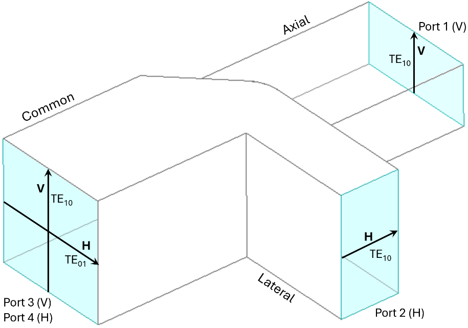
Figure 1 – Simplified asymmetric T-Junction OMT with polarization and port designations.
Difficulties of Characterizing OMTs
RF testing of OMTs is complicated by the presence of the common mode port, which supports two orthogonal modes. Vector network analyzers have single-mode test ports. The question is how to handle the common-mode port in testing.
Testing with a Short Circuit Termination on the Common Mode Port
The easiest way to test an OMT is by terminating the common mode waveguide (port 3 and port 4) with a short circuit (a flat metal plate). Short-circuit terminations for rectangular waveguides are readily available in calibration kits and work equally well on square waveguides. Using the short circuit termination, we can measure the OMT insertion loss. A signal flow graph is shown in Figure 2. Port 1 and port 2 are single-mode rectangular waveguides and can be attached to a vector network analyzer.
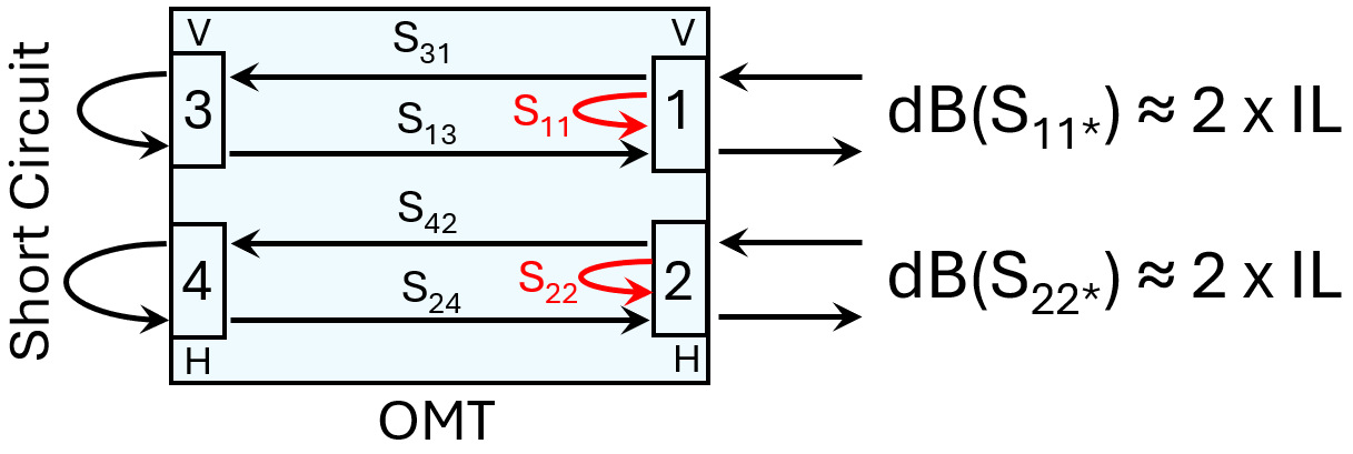
Figure 2 – Signal flow graph showing how insertion loss is measured using a short circuit termination on the common mode port. Note: dB(S11*) = 20 × log(S11*).
The characteristic OMT reflections S11 and S22 are defined when all ports are terminated in a matched load. We use the terms S11* and S22* to designate the reflections observed at ports 1 and 2 when the common-mode waveguide port is terminated with a short circuit. S11 ≠ S11* and S22 ≠ S22*.
Consider a signal incident on port 1. Most of the signal propagates through the OMT, is coupled to port 3, is reflected at the short circuit termination, and returns to port 1. For now, we will ignore the impact of cross-polarization coupling and isolation. We assume they will have little impact on the measured values of dB(S11*) and dB(S22*) since they are orders of magnitude smaller than the characteristic OMT insertion losses -dB(S31), -dB(S13), -dB(S42), and -dB(S24). The characteristic OMT port reflections dB(S11) and dB(S22) are also assumed to be low (near -20 dB). Under these conditions, the measured value dB(S11*) ≈ dB(S31) + dB(S13) and the measured value dB(S22*) ≈ dB(S42) + dB(S24). Therefore, the measured port reflections are approximately equal to two times the insertion loss (IL).
We now consider the measured data dB(S21*). The signal flow graph in Figure 3 shows three distinct signal paths for a signal entering port 1 and exiting at port 2. Most of the signal incident from port 1 reaches port 3. But when the signal reflects on the short circuit termination, some of the signal does not return to port 1 but rather is cross-polarization coupled to port 2. This is the scattering parameter S23. If the OMT is working properly, dB(S23) will be very small, perhaps at the -40 dB level as indicated in Figure 3.

Figure 3 – Signal flow graph for an OMT with a short circuit termination on the common mode port. (Modified from Alessandro Navarrini and Renzo Nesti [4]).
Some of the incident signals from port 1 never reach port 3 but rather are cross-polarization coupled to port 4. The cross-polarized signal reflects at the short circuit termination and is then coupled to port 2. The associated S-parameter is S41. And lastly, a portion of the signal incident on port 1 is directly coupled to port 2. The associated S-parameter is S21 (isolation = -dB(S21)). We have neglected the insertion loss terms S31 and S24 for the sake of simplicity. The same analysis can be made for an excitation on port 2, yielding an aggregate signal at port 1, dB(S12*). In this case, the signal exiting at port 1 comprises the isolation term S12 and the cross-polarization terms S32 and S14.
The signal flow graph in Figure 3 shows that the isolation and cross-polarization data are intermixed in the signal exiting at port 2. But some useful information can be extracted from the data. We don’t know the exact magnitude of any of the three S-parameters, S21, S23 and S41, but we can establish a maximum value for all three. If the aggregate signal exiting at port 2 is at the -40 dB level, then we know that the isolation must be greater than 40 dB and the cross-polarization coupling must be less than -40 dB. If any of the three scattering parameters S21, S23, or S41 were worse than -40 dB, it would dominate the measurement. For example, if the isolation term dB(S21) were at the -30 dB level and the cross-polarization coupling terms, dB(S23) and dB(S41), were -40 dB, the aggregate signal exiting the OMT at port 2 would be at the -30 dB level.
RF Testing Takeaways
RF testing OMTs is complicated by the presence of the common mode port, which cannot be connected to a network analyzer. But it is possible to measure the insertion loss and to get qualitative data for the cross-polarization coupling and isolation by terminating the common mode port with a short circuit (a flat metal plate). This is the easiest type of measurement to make in the laboratory since short circuit terminations are commercially available and included in many calibration kits. In fact, the exact waveguide band does not matter so long as the short circuit can be mated to the common mode flange. For example, a WR-12 short circuit termination can be used on the common mode port of WR-3.4 OMT since the two flanges mate.
In the next two blogs in this series, we will look at testing OMTs with matched loads and testing in back-to-back configurations using two OMTs connected at the common mode ports. These tests can provide accurate data for port reflections as well as cross-polarization coupling and isolation.
At MicroHarmonics, we design and manufacture high-precision RF components, including orthomode transducers, attenuators, isolators, and circulators. These products are engineered to provide reliable, accurate measurements for advanced RF and microwave applications, making them essential tools for laboratories, research institutions, and high-frequency test environments. If you have any questions about our products, please contact us.
References
[1] D. Porterfield, “Orthomode Transducers: Part 1 – Introduction and Applications,” A brief description of orthomode transducers (OMTs) and common applications. https://microharmonics.com/blog/, January 31, 2025.
[2] D. Porterfield, “Orthomode Transducers: Part 2 – Architectures,” A brief description of some of the most common mm-wave OMT architectures. https://microharmonics.com/blog/, May 21, 2025
[3] D. Porterfield, “Orthomode Transducers: Part 3 – Characterization,” A description of important OMT parameters including insertion loss, port reflections, cross-polarization coupling, and isolation. https://microharmonics.com/blog/, 2026
[4] Alessandro Navarrini and Renzo Nesti, “Characterization Techniques of Millimeter-Wave Orthomode Transducers (OMTs),” Electronics 2021, Vol 10, Issue 15, 1844, https://doi.org/10.3390/electronics10151844.