Orthomode Transducers: Part 3 – Characterization

David W. Porterfield, PhD
Founder, Micro Harmonics

In previous blogs, “Orthomode Transducers: Part 1 – Introduction and Applications” and “Orthomode Transducers: Part 2 – Architectures“, we gave a brief description of orthomode transducers (OMTs), discussed some applications, and described some basic architectures. In this third post, we will examine the important characteristics of OMTs and explain why it is difficult to accurately measure the RF performance. We will also describe some practical methods to characterize OMTs.

OMT Description

OMTs have three waveguide ports. Two of the ports support a single propagating mode, typically the TE₁₀ mode in a rectangular waveguide. The third port, often referred to as the common mode port, supports two orthogonal propagating modes. The common mode waveguide can have a square cross-section supporting the orthogonal TE₁₀ and TE₀₁ modes [1-5] or a circular cross-section supporting a pair of degenerate orthogonal TE₁₁ modes [6, 7].

Figure 1 shows a simplified sketch of an OMT. Port 1 on the axial waveguide and port 2 on the lateral waveguide each support a single TE₁₀ mode. The common-mode waveguide supports two polarizations designated as vertical (V) and horizontal (H). The two modes can be treated as two distinct ports, port 3(V) and port 4(H). The vertical (V) and horizontal (H) designations simply help us keep track of the associated polarizations. An ideal OMT couples 100% of the vertically polarized signal from port 1(V) to port 3(V) and 100% of the horizontally polarized signal from port 2(H) to port 4(H).

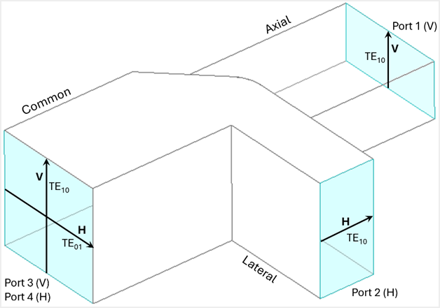
Figure 1 – Simplified asymmetric T-Junction OMT.

Important Characteristics of OMTs

OMTs are reciprocal networks since they are passive and comprise isotropic materials. In a reciprocal network, transmission coefficients between two ports are identical regardless of which direction the signal propagates. The magnitudes of the port reflections are also equal at opposite ports for the two polarizations. Using the port designations in Figure 1, we can establish the following relationships.

S₁₃ = S₃₁    S₂₄ = S₄₂    (insertion loss)    Equation 1

S₁₄ = S₄₁    S₂₃ = S₃₂    (cross-polarization coupling)    Equation 2

S₁₂ = S₂₁    (isolation)    Equation 3

|S₁₁| = |S₃₃|    |S₂₂| = |S₄₄|    (port reflections)    Equation 4

Insertion Loss

Insertion loss refers to how much the vertically or horizontally polarized signals are attenuated as they pass through the OMT. Attenuation is primarily caused by conductor losses in the OMT waveguides. Many OMT structures have asymmetry between the axial and lateral waveguides, so the insertion losses differ for signals in the two polarizations. Using the Figure 1 port designations, the insertion loss for the vertically polarized signal is given by Equation 5, where T is the transmission coefficient.

Insertion Loss = −20 log T = −20 log |S₃₁| = −dBS₃₁    Equation 5

Equation 1 shows that −dB(S₁₃) = −dB(S₃₁). The insertion loss for the horizontally polarized signal is given by −dB(S₄₂) or −dB(S₂₄).

Low insertion loss is critical because OMTs are typically positioned at the antenna feed. This places them in front of the first low noise amplifier, where losses can significantly degrade the system noise figure. Insertion losses generally increase at higher frequencies. As a point of reference, the Micro Harmonics WR-3.4 OMT [8] has an insertion loss of less than 0.8 dB in both polarizations across the full waveguide band from 220–330 GHz.

Isolation

Isolation is defined between the axial and lateral waveguide ports when there is a matched load on the common mode port. Using the port designations in Figure 1, the isolation is given by −dB(S₁₂) and −dB(S₂₁). Ideally, there is no coupling between these ports, but in practice, some leakage occurs. The Micro Harmonics WR-3.4 OMT [8] has a measured isolation of approximately 50 dB across the band 220–330 GHz.

Cross-Polarization Coupling

Some of the vertically polarized signal on port 1(V) gets coupled to the horizontal polarization on port 4(H). The relevant S-parameter designations are dB(S₁₄) and dB(S₄₁). Cross-polarization coupling also occurs between the horizontal polarization on port 2(H) and the vertical polarization on port 3(V). The relevant S-parameter designations are dB(S₂₃) and dB(S₃₂). Cross-polarization coupling is often abbreviated as cross-pol coupling, cross-pol, or simply XPC.

An ideal OMT has zero cross-polarization coupling. The very purpose of the OMT is to separate and distinguish between the two polarizations. But in practice, cross-polarization coupling is non-zero due to asymmetries, misalignments, machining errors, and limitations in the OMT architectures. As a point of reference, the Micro Harmonics WR-3.4 OMT [8] has a measured cross-polarization coupling of less than −38 dB across the 220–330 GHz band (less than 0.016% of the signal is coupled to the wrong port).

Port Reflections

The port reflections on the OMT are given by S₁₁, S₂₂, S₃₃, and S₄₄. Low port reflections are essential for the proper operation of most microwave and millimeter-wave components. The implicit assumption is that the component accepts the incident signal and does something useful with it rather than simply reflecting it. Port reflections can cause standing waves in high-frequency microwave and millimeter-wave systems. These standing waves negatively impact bandwidth and system performance.

Building on these key orthomode transducer characteristics, Micro Harmonics applies rigorous design, manufacturing, and testing to ensure low insertion loss, high isolation, minimal cross-polarization coupling, and controlled port reflections across all its components. In addition to precision orthomode transducers, the company offers high-performance isolators, circulators, and variable attenuators, all engineered for demanding millimeter-wave applications. These components allow engineers to achieve accurate RF performance even in the most challenging system environments.

To explore Micro Harmonics products or discuss a custom solution for your application, contact our team for expert guidance.

References

[1] A. Dunning, S. Srikanth, and A. R. Kerr, “A simple orthomode transducer for centimeter to submillimeter wavelengths,” in Proc. Int. Symp. Space Terahertz Technol., Charlottesville, VA, Apr. 2009, pp. 191–194.

[2] T. J. Reck and G. Chattopadhyay, “A 600 GHz asymmetrical orthogonal mode transducer,” IEEE Microw. Wireless Compon. Lett., vol. 23, no. 11, pp 569–571, Nov. 2013.

[3] A. M. Bøifot, E. Lier, and T. Schaug-Pettersen, “Simple and broadband orthomode transducer (antenna feed),” in Proc. IEE H-Microw. Antennas and Propag., vol. 137, no. 6, pp. 396–400, Dec. 1990.

[4] A. Navarrini and R. Nesti, “Symmetric reverse-coupling waveguide orthomode transducer for the 3-mm band,” IEEE Trans. Microw. Theory Techn., vol. 57, no. 1, pp. 80–88, Jan. 2009.

[5] T.-L. Zhang, Z.-H. Yan, L. Chen, and F.-F. Fan, “Design of broadband orthomode transducer based on double ridged waveguide,” in Proc. Int. Conf. Microw. Millim. Wave Technol. (ICMMT), May 2010, pp. 765–768.

[6] A. Navarrini and R. L. Plambeck, “A turnstile junction waveguide orthomode transducer,” in IEEE Trans. Microw. Theory Tech., vol. 54, no. 1, pp. 272–277, Jan. 2006.

[7] G. Pisano et al., “A broadband WR10 turnstile junction orthomode transducer,” IEEE Microw. Wireless Compon. Lett., vol. 17, no. 4, pp. 286–288, Apr. 2007.

[8] Micro Harmonics Corporation, WR-3.4 Orthomode Transducer, https://microharmonics.com/millimeter-wave-orthomode-transducers/